
David J. Hartshorne
The New Science of Fixing Things has developed a reputation as a group of extraordinary technical problem solvers. We are the company that is called on when others have struggled. Are we smarter than others, or have we learned some important principles over the 30 years of working together on tough problems? Well, we think that some principles are so important that we put all our effort into making sure cover them at the beginning of a project. There are others, but some key ones are:
- Only ever employ a progressive search that is based on a small set of simple models of systems, all of which can be expanded top-down when needed. The models are far more important than any tools used to analyse System Behaviour.
- Ensure we are able to see what’s happening during a single cycle or operation of the device or system (after Galileo with his ball and ramp)
- Have a goal to reach a Causal Explanation of behaviour rather than a root cause linked to a problem.
- When characterizing behaviour, ensure that all observations we make capture how well the machine is working AND that any single observation we make carries as much explanatory information as possible.
- Individual devices within systems all manage energy in some way, and often the most efficient and effective way of getting to a Casual Explanation (sometimes the only way) is to characterize what happens to energy.
A problem with principles is that compressing them into a few words is great for checking the box, but not for capturing their real meaning or importance.
In order to illustrate them better, we thought it may be a good idea to explain how they apply to understanding a simple device that a lot of people are not only familiar with, but also will have analysed its behaviour in some detail as part of their six sigma training. That device is the mangonel catapult used to demonstrate design, analysis and interpretation of experiments to understand the effects a number of different variables have on a response, which is usually determined during the project definition phase of the exercise to be the range achieved when the catapult fires a ball. I first saw a version of this in the mid 1980s. Here is a sketch of one currently in use:
The factors or variables that can be adjusted include:
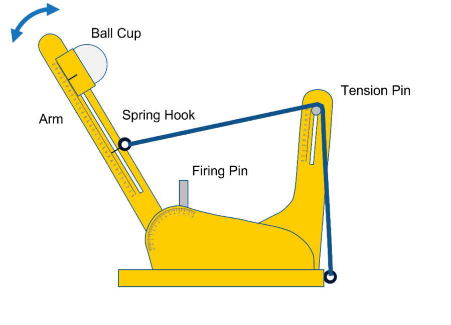
A Release angle
B Tension pin height
C Firing angle
D Hook position
E Cup position
F Ball type (2 colors)
G Bungee type (2 colors)
The exercise provides the opportunity to show the application of a number of sophisticated experimental designs such as two-level fractional factorials or Plackett-Burmann designs, all with the objective of separating or screening out the trivial many from the vital few factors. This requires a dozen or so tests (to satisfy criteria on degrees of freedom) to be conducted at levels of the factors chosen by brainstorming. This phase is typically followed by a full factorial experiment on up to four factors deemed to be either important or not well enough understood, possibly at new levels or settings. This phase typically involves sixteen further individual tests covering every combination of factors. For example, if the brown bungee type, highest cup position and pink ball always give best results these factors can’t be studied further, leaving A, B, C, and D to be tested. A full factorial design ensures that interactions or interdependencies between factors are also tested.
Analysis of the results and testing if an effect is bigger than “noise” has to be conducted, which can be quite tedious when done manually, and so today software is usually employed.
The exercise might, for example, screen out factors E, F and G because ball and bungee type and cup position are overwhelmingly important. Then, depending on the actual factors, and the levels or settings tested, the outcome might look something like this:
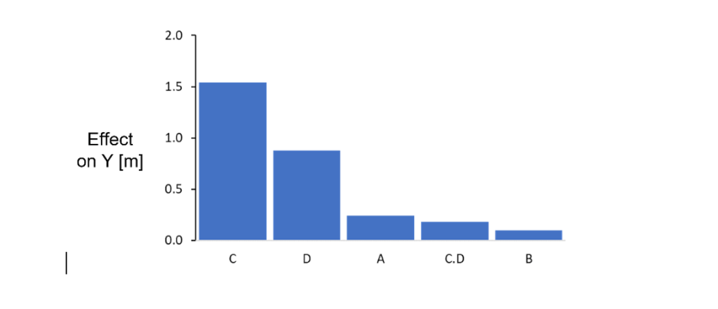
Based on that outcome we might say that the bungee type and cup position are critical design factors, and that hook position and firing angle are root causes of variation in range achieved firing the ball. Type of ball might be considered an input factor.
The entire approach to such a study of behaviour of the catapult, ending with these statements is based on a very specific model of the world, which we call the Black Box model.
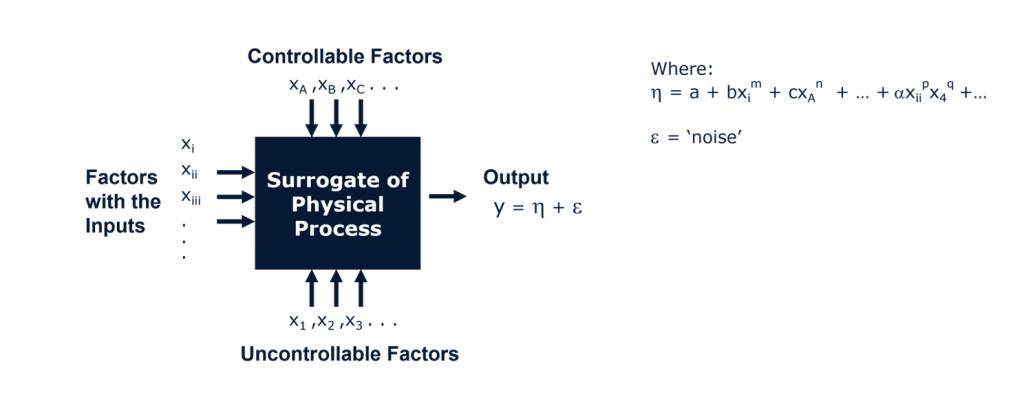
If the factors are continuous variables as opposed to things like pink ball vs yellow ball, green bungee vs brown bungee, then the response can be written as a function of the factors like this:
Y = 6.611 – 0.012.A + 3.850.B – 0.077.C + 7.645.D – 0.033.C.D + noise
which is a specific expression of that algebraic model. Whilst it is useful for predicting and optimizing the firing range of the specific catapult arrangement being studied, within the operating range tested, it doesn’t really tell us how the system works, how we can best exploit it, and what we can do to make it better. This is particularly important if the optimized performance is still marginal with some balls still falling short of their target, or not doing any damage when they hit it. It doesn’t give us insight. For example, what is the mysterious source of variation that occurs when the positions of B, C and D are changed in the experiment?
If we hold the approach to this exercise up against the principles we believe are so important, it doesn’t seem to do very well. If the exercise was conducted in a real factory or engineering centre on a real product, it would also represent a considerable investment in resources and time.
The model that the whole approach is based on is undoubtedly useful. We periodically fall back on it when, even using the correct characterization, the search space still needs reducing efficiently and effectively before we are able to state the Causal Explanation for a system’s behaviour.
There is however, a different model that is more appropriate to use for the catapult and a lot of real-world machine systems. It also helps us stick to our important principles.
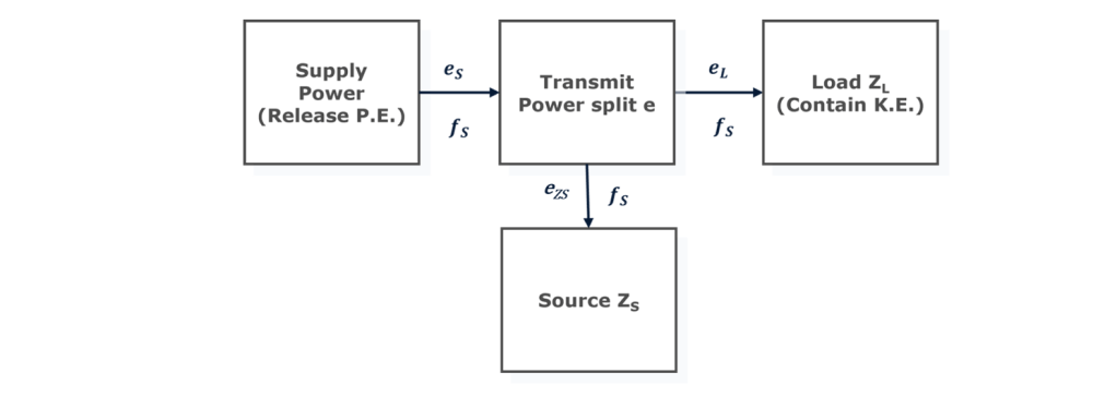
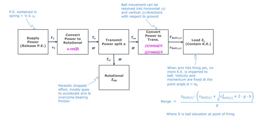
This is a functional model depicting how and why energy is used. At the highest level shown here, it is as general in application as the Black Box model shown earlier. It says that there is a source of energy, a load impedance the purpose of which could be to contain energy in a different form or simply to dissipate the energy in a way that is useful to us, or both. Between the source and the load is a means of controlling release of the energy from the source and transmitting energy to the load. There is also has an additional impedance associated with the source leading to dissipation and energy storage which is parasitic. The arrows between the boxes represent the flow of energy, the rate at which that happens is power.
Whilst the Black Box model as we drew it above is expressed in terms of function and inputs, it is not really a functional model, and factors that belong with either the function or the inputs (which really means stuff made of matter, not energy) are most often looked at structurally – quantifying the contributions made by the pieces from which a system is made rather than directly characterizing what it does and how it works. However sophisticated the analysis, the Black Box model is fundamentally restricted to statements about root causes.
To relate the catapult to the Source-Load model we can see that there is a potential energy source which is the bungee spring that is stretched by the operator prior to release. The load is the ball, the main impedance property being its mass. The primary function is really to contain kinetic energy in the ball for subsequent release by smashing it into a target and doing as much damage as possible. This may not accord with the problem which has been defined as fire the ball the longest distance. If the objective is to destroy a target, the task would be to launch a repeatable distance with maximum kinetic energy.
Let’s now consider how we characterize behaviour to maximize what we learn as quickly as we can. In the generic Source-Load model, the arrows are each associated with a conjugated pair of generalized variables; an effort and a flow. In all of the different manifestations of energy such as electrical, rotary motion, chemical and so on there will be an effort and a flow measurable in appropriate units. Whenever a source’s effort exceeds a load’s opposing effort, the difference induces a flow as the system moves towards equilibrium. In the case where the effort results from a difference in force, the flow is a translational motion in a straight line and is measured in units of distance per unit time. To quantify both energy and power we need to quantify the appropriate conjugate variables. Power is always effort multiplied by flow for example. Keeping track of them separately is one of the best ways of maximizing information about what’s happening.
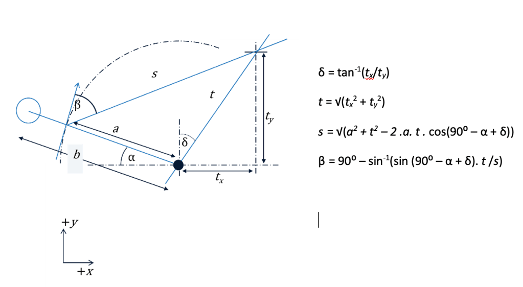
Before we can start filling in details about what are the specific conjugate variables that are associated with a power branch we would like to characterize, and how we might obtain them, we start with a basic cartoon to capture the key elements of a mechanism – what should determine how the mechanism or device releases, converts, transmits, contains or dissipates energy. In this case it is a few geometrical relationships that define how some of the functions operate.
Using the cartoon we can see that we need to know the extension of the spring s and the angle β between the limits of α which are -20⁰ to 120⁰
a = arm length controlled by Hook Position
b = is controlled by Ball Cup Position
ty is controlled by Tension Pin Position
tx is fixed by the dimensions of the catapult
The release angle αR must clearly be less than the firing angle αF
For any spring, in fact any potential energy storage device, the energy contained is characterized by the conjugates effort and displacement – notice that flow variables are displacements divided by unit time and while potential energy is being contained or released the displacement changes with time.
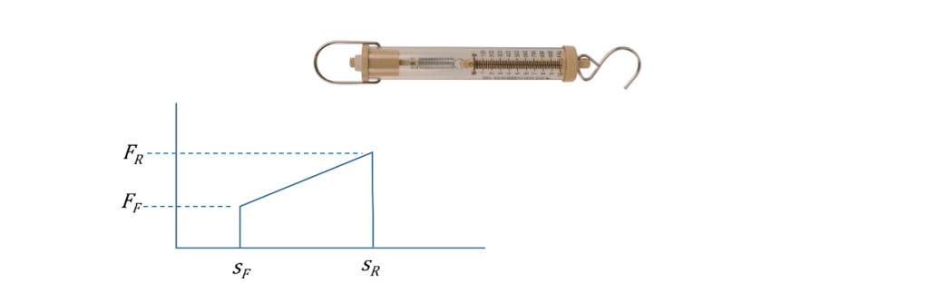
For $10 we can buy a force gage or calibrated fish hook which we can use to characterize the energy contained in the spring as it is extended by moving the arm from the firing position to the release position, taking care to hold the gage in line with the bungee in both positions. Alternatively, we can ensure it is kept perpendicular to the arm and base our calculations on torque. This gives us effort on the input side, but what about flow?
On the load side, because it is a kinetic energy storage device, the ball will have a changing velocity for the time it is in the cup, and a final velocity at the point of firing when the arm is stopped. The force applied to the ball via the arm accumulates between release and firing. This accumulation of incremental effort multiplied by incremental time units is the conjugate to flow for characterizing kinetic energy when its being contained or released and is called momentum. For motion in a straight line this happens to be also equal to mass multiplied by velocity, leading to the familiar expression for kinetic energy of mv2/2. We do need to know the mass of any ball we fire if we want to understand the full picture, but that is easy.
Knowing the velocity and the ball height and angle of inclination at firing (which are both adjustable on the catapult and important due to the effect of gravity) fixes the range or flight distance. Of course, putting the catapult on a table has a big effect on range. Nevertheless, if we know the other two parameters, knowing the distance is the same as knowing the velocity at firing by doing a little algebra). So flight distance isn’t such a bad response for characterizing the catapult behaviour. But what about the conjugate to velocity; the force on the output side? Well, if we knew how long it had taken to travel from release to firing position we could get a rough idea using F=ma, and with a little geometry we can compare the output force to the input force and see how well the device works. An app that makes use of the accelerometers in your phone can time such short events crudely, but there is additional information from another measurement we could make that we will mention later.
Importantly, using the Source-Load thinking model, we can see that the adjustable factors considered in the DoE are in fact split between different functions. If we stick with the goal being to maximize range, the elevation and inclination are important independent of how much energy is supplied or the load impedance (mass of the ball). There is an optimum firing angle and that is that. The higher the elevation above the target at firing, the further any ball will travel.
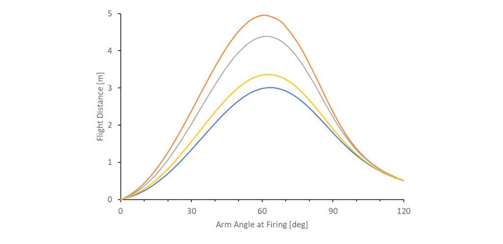
Optimum firing angle is independent of how much energy the ball has
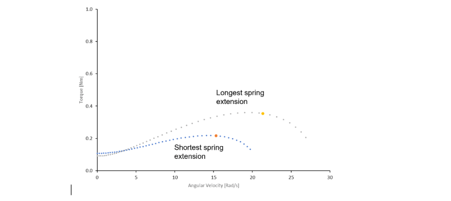
A lot of information about what is happening is available in a simple plot of effort vs flow on the power branch going to the load. The characteristic curves for both sources and loads can be added based on just half a dozen data points. There is a lot of knowledge about what is happening to be gained from this plot. We have added six additional data points from the tests conducted during the DoE. Everything on the plot is fired at 70⁰. Tests fired at 90⁰ will have passed through these points at 70⁰, but more about that later.
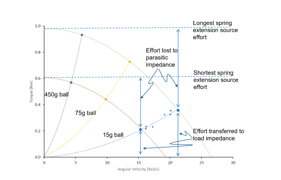
Using the geometry from the cartoon, we converted the results into rotary motion conjugates; torque and angular velocity, because that’s where the action is. We can see that the greater the mass of the ball, the more force that is required to accelerate it, or for the same force a lower acceleration is achieved meaning a lower velocity at firing, leading to a shorter range.
Every other adjustable factor affects how much energy is contained in the spring prior to release, and so we should seek to maximize that function whatever the individual contributions are. For the catapult, more energy in means more energy out in spite of heavy losses.
The major parasitic energy loss is greater than the energy imparted to the lighter balls, so a longer range comes at a high price. That loss is initially contained as kinetic energy in the arm, but is dissipated when the arm hits the firing pin. There is some small loss in the arm’s bearing too, but a major performance improvement comes from having an arm that is as light as possible as long as it is stiff enough..
Characterizing the energy contained in the stretched bungee spring using the force gage also revealed that the spring pre-load and spring rates varied depending on how the bungee spring was positioned prior to tensioning. Looping the bungee round an adjustable peg may have been an intentional ploy of the catapult designer in order to build in a hidden source of noise to the exercise. Perhaps we should have given a spoiler alert at the very start.
For $10 and an additional thinking model we can figure out a lot about what’s happening with the catapult, and the Causal Explanation has a much broader application to catapult design and operation than a Black Box model that is merely pretty good at predicting the flight distance. We can do it in a fraction of the time it takes to conduct and analyse even the best designed and executed DoE tests, or if we choose, explain the DoE results as well as solving the mystery of poor repeatability from different set-ups even when a single set-up repeated nicely. Such an outcome happens with real machines in the real world all the time to us, and is how we have achieved our reputation.
The only one of the principles outlined at the beginning that we haven’t fully stuck to is the one that talks about looking deeper into what’s happening during a single operation of the catapult (as Galileo would have). To do that, and to get a more accurate characterization and an even deeper understanding of what’s happening, we would need a rotary motion sensor and data acquisition software on a laptop, costing about a couple of hundred dollars. Such a sensor provides angular displacement, velocity and acceleration data. With a little geometry, a full picture of the effort-flow, effort-displacement or momentum-flow conjugates associated with every branch at each time step can be obtained.
The Source-Load model could be slightly expanded to include the energy conversion from translational motion to rotary motion and then back again to translational, since the major parasitic impedances are in the rotational domain.
Effort-flow between release and firing as late as 120⁰. 70⁰ point is highlighted.
In real world machines today, typically most if not all the sensors we need are built in, and the raw data is very useful. The problem is that most of the time software compresses the data, stripping it if its information content, then storing the data which no longer has any value for hundreds of thousands of cycles. Because the data is there, those tasked with solving problems are compelled to analyse it six ways to breakfast, but the important information is not displayed…but it is there!
DoE has its place, but for decomposition of machine behavior where the operation is based upon the flow of energy and power, The Source Load model provides the best insight into performance and reliability improvement. When used for for product performance characterization, you will gain a new level of confidence about the products you make and sell.
David J. Hartshorne
Posted and edited by John Allen
